Assessing normality
An assumption that data are normally distributed underlies many of the commonly used statistical techniques. Therefore, statisticians need to be able to assess whether the data in a sample do indeed follow a normal distribution. Two common ways of doing this are the Shapiro–Wilk test and the Kolmogorov–Smirnov test. Running the Shapiro–Wilk test on the data set in Table 33.1 gives P = 0.978, (an explanation of P is given later in this chapter), showing that the data do not deviate significantly from a normal distribution.
| Ranked data (kg) | Grouped data | |
|---|---|---|
| Weight range (kg) | Number | |
| 42, 46, 46, 49, 50, 50, 51, 53, 54, 54, 55, 56, 56, 56, 57, 58, 59, 59, 60, 60, 61, 61, 62, 62, 62, 63, 64, 64, 65, 66, 67, 67, 68, 68, 69, 70, 70, 72, 74, 75, 76, 77, 78, 80, 84 | 38–42 | 1 |
| 43–47 | 2 | |
| 48–52 | 4 | |
| 53–57 | 8 | |
| 58–62 | 10 | |
| 63–67 | 7 | |
| 68–72 | 6 | |
| 73–77 | 4 | |
| 78–82 | 2 | |
| 83–87 | 1 | |
Incidentally, it is possible for a distribution to be symmetrical but not normal; this can happen if the distribution is very widely distributed around the mean (i.e. flat) or very closely grouped around it, so the distribution is tall and thin. The ‘peakedness’ of distributions, both normal and non-normal, can be measured by calculating the kurtosis.
Range
Range is the spread of data in a sample. In Table 33.1, the range is 42–84 kg. The range is especially unhelpful when a data set is skewed.
Mode or modal group
The mode is the value that occurs most frequently in a data set. The modal group is the interval on a frequency histogram within which the greatest number of observations fall. In Figure 33.1, the modal group is 58–62 kg.
It is worth remembering that some data will have two or more peaks in their distribution. Always look critically at a frequency histogram to see whether there is evidence for a multimodal distribution.
Median
The median is the middle value in a ranked data set. The median is much less influenced by skewed data sets than the mean.
Find the median of 5, 1, 8, 3, 4:
First sort the measurements (put them in order): 1, 3, 4, 5, 8.
The median is the (n + 1)/2th value in the set, where n is the number of observations.
In this set, the median is the third value, i.e. 4 (not 3).
Mean
The mean is the statistician’s term for an average  .
.
Mean

where ∑ = ‘the sum of’, x = each individual observation and n = the number of observations.
Quantifying Variability (Scatter) in a Normal Distribution
Variance
By itself, variability is not very helpful in describing the ‘average’ family, as the same mean as for example 3 could have been arrived at if the families had had 2, 2, 2, 3, 3 and 3 children. To illustrate the differences in the data, an estimate of the scatter in the sample is needed. Variance is the average amount by which any individual measurement differs from the mean.
Variance
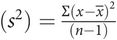
Standard deviation
Standard deviation (s or SD) is the square root of the variance (in original units). It is used because some of the differences will be positive, and some negative and, if the squaring were not carried out when calculating the variance, some differences would cancel others out, which would be logically useless. The standard deviation gives information about the scatter in a sample.
Statisticians describe the population mean and standard deviation as µ and σ, respectively. This is different from the sample mean  and standard deviation (s).
When data from a population can be described by a normal curve:
The area covered by ± 1 σ from µ = 68%. This means that 32% of the area lies more than ± 1 σ away from the mean. Because the distribution is symmetrical, 16% lies to the left of µ and 16% to the right of it.
The area covered by ± 2 σ from µ = 95%. Thus 5% lie outside this range, with 2.5% in each ‘tail’.
The area covered by ± 3 σ from µ = 99.8%. What proportion lies outside this range?
In a normally distributed sample with 30 or more observations (n ≥ 30), the same approximations can be used for the sample mean  and standard deviation (s).
In Figure 33.2, any position on the x axis can be described by how many standard deviations (the distance) it is away from the mean, on either side. This distance is known as the normal (z) score or standard normal deviate. All statistical textbooks have tables of z scores.
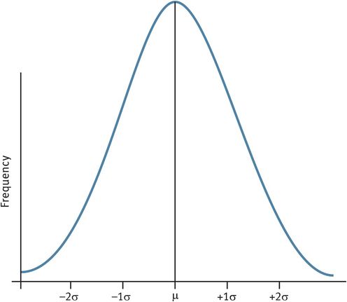
The normal distribution curve
Coefficient of variation
The coefficient of variation expresses the standard deviation as a percentage of the mean.
Coefficient of variation
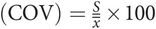
This is useful, for example, in quantifying the reliability of repeated measurements, since it puts the standard deviation in the context of the mean.
Standard error of the mean
The standard error of the mean (SEM) gives information on how close a sample mean is to the population mean. If several samples from a population were taken, each sample would have its own mean and variance and only by chance would the sample mean be the same as the population mean. In a normally distributed population, these sample means would themselves have a normal distribution. Calculating the mean of those sample means would usually give a better idea of the true population mean, so the variability of this distribution of sample means is assessed by calculating their standard deviation. This is known as the SEM. The smaller the SEM is, the closer the sample mean lies to the population mean. It is derived from the standard deviation (s) and the sample size (n).
SEM =
 or SEM =
Arithmetically, these formulae are the same.
The SEM thus takes into account both the scatter and the sample size, thus allowing for the fact that the mean of a bigger sample will be more representative of the true population mean than will the mean of a smaller sample.
Let the mean  booking weight in a sample = 52 kg and the standard deviation (s) = 12 kg:
If n = 9, SEM = 12 /√9 = 12/3 = 4 kg.
If n = 16, SEM = 12 /√16 = 12/4 = 3 kg.
If n = 100, SEM = 12 /√100 = 12/10 = 1.2 kg.
Confidence intervals
For a normally distributed sample with 30 or more observations (n ≥ 30), the same assumptions about the areas under the normal curve can be used for the sample mean, x–, and standard deviation, s, as for the population mean, µ, and standard deviation, σ. These allow the calculation of confidence intervals describing the distribution of data in the sample.
Let the mean booking weight in a sample of n = 36 be 52 kg and the SEM be 3 kg:
95% CI = 52 ± (2 × 3) = 52 ± 6 = 46–58 kg.
The practical interpretation of this is that, in this example, there is a 95% probability that the true population mean lies between 46 and 52 kg (or a 5% probability of the true population mean lying outside this range).
Skewed Data
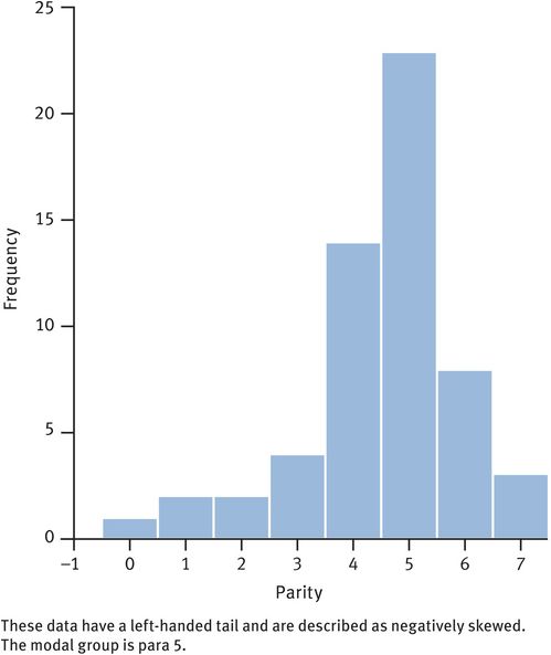
The distribution of positively skewed and negatively skewed samples are shown in Figures 33.3 and 33.4. The effect of the skewness is to make the mean less ‘typical’ than other measures that are less influenced by extreme values, such as the median. However, the SEM can still be used for confidence limits because, even with skewed data, the distribution of sample means approaches a normal distribution.
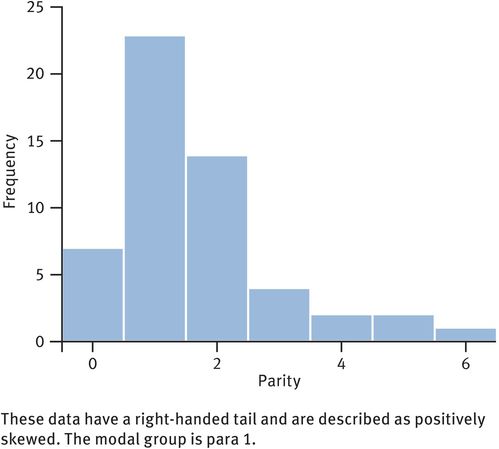
Frequency histogram of parity from a sample of women in an area where large family size is the norm
Consider a sample of six women with different parities (number of pregnancies leading to a successful outcome after 20 weeks of gestation): para 4, para 2, para 1, para 3, para 2 and para 3:
Mean parity is 2.5.
Variance is 1.1.
s is 1.05.
SEM is 0.43.
In a larger sample of 53 women (Figure 33.3), 7 were para 0, 23 were para 1, 14 were para 2, 4 were para 3, 2 were para 4, 2 were para 5 and 1 was para 6:
Median parity is the (53 + 1)/2th value in the ranked set, i.e. the 27th value.
Since there are 7 para 0 and 23 para 1, the 27th value must be para 1.
Normalising skewed data
When data are not normally distributed, it may be possible to transform them to a normal distribution. This allows the correct use of the mean, standard deviation and standard error of the mean for each sample and thus the calculation of confidence intervals. It also allows the use of more powerful comparative statistics for hypothesis testing.
Endocrine data often follow a positively skewed distribution. This can be normalised by taking the logarithm of the data.
Other commonly used transformations are:
taking the square root (√x)
squaring (x2)
taking the reciprocal (
 ).
).
The Binomial Distribution
The binomial distribution is the simplest form of distribution. It is used for data measured on a discontinuous dichotomous scale (for example, yes/no, alive/dead). With dichotomies, if the proportion (p) of subjects falling into one category is known, the proportion in the other, which is (1 – p) or q, is automatically known.
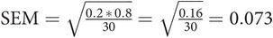
When the number of observations is more than 30 (n > 30), the binomial distribution approximates to the normal distribution, which is very useful. Under these circumstances, the standard deviation of p is given by p × (1 – p) and the standard error:
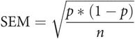
This can be used to establish confidence intervals for p.
In a sample of 100 pregnant women, 20 admitted smoking; therefore p = 0.2 and (1 – p) = 0.8:
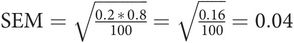
There is only 1 chance in 20 of the true population proportion of smokers lying outside the range:
95% CI = 0.2 ± (2 × 0.04) = 0.12–0.28, or 12–28%.
The Poisson distribution
This is another kind of distribution of discrete data, arising when the number of occurrences of an event per unit of time are counted. It therefore relates to integers (whole numbers). This type of distribution was first described by a Prussian army statistician (Figure 33.5). A modern example of the distribution could be the number of admissions to a gynaecological unit from the accident and emergency department each day. Over a period, an average number of admissions can be calculated, but the actual number of admissions each day will be randomly variable. The Poisson distribution allows the calculation of the probability of any specified number of admissions on a single day. Thus this is useful when considering random sums of rare events.
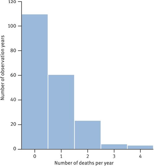
Frequency histogram of the number of deaths/year in the Prussian Army caused by being kicked by a horse
With a Poisson distribution, the distribution is skewed when the mean is close to zero, but the distribution approximates to normal as the mean increases. If the mean number of events is around 9, then the normal approximation is reasonable.
The variance in a Poisson distribution is the same as the mean, so:
Probability
The probability of a specific outcome is the proportion of times that the outcome would occur if the observation or experiment was repeated a large number of times.
Comparative statistics and hypothesis testing
So far in this chapter, descriptive statistics have been considered. Another important branch of statistics is comparative statistics. These are used when comparing, for example, the effect of a fixed variable, such as gender on a disease or condition, or determining whether some intervention has an effect on a disease or condition. Under both circumstances, hypothesis testing works, by convention, from a null hypothesis (H0), which states that the variable is without effect, and then testing the null hypothesis.
The probability of any observed outcome arising if the null hypothesis is valid is calculated and used to support or reject the hypothesis. This probability is referred to as the P value and the smaller P is, the less can the null hypothesis be supported. The P value can be defined as the probability of having observed any specified outcome (or one more extreme) if the null hypothesis is valid.
By convention (and it is only by convention), H0 is usually rejected if P < 0.05. That is, an outcome causing rejection of H0 could occur less than one time in 20 even when the H0 was valid.
The use of P values is open to two main errors:
Always remember that statistical and biological significance need not be the same. Large studies can make very small differences statistically significant, while even large biological effects can be statistically nonsignificant in a small study. So do not rely too much on P values. The difference between P = 0.053 and P = 0.047 may technically be the difference between acceptance and rejection of the null hypothesis but should not constrain thinking about possible implications of erroneously stating that there is no effect.
Sample Size Determination
When any study is being designed, the size of sample is very important. It must be big enough to give a high chance of any real difference being identified as statist-ically significant. This should be governed by taking both alpha and beta errors into account.
The power of a study is its ability to detect an effect of a specified size. It is expressed as (1 – β) or 100(1 – β)%.
The sample size (n) is usually calculated to give a power of 0.8–0.9 (80–90%). For any hypothesis test, alpha is set in advance (usually 5%) so P < 0.05 supports rejection of H0.
Types of Test for Hypothesis Testing
The type of data that is collected will determine what forms of analysis it can be subjected to. Are the data nominal (categorical), ordinal, discrete (integers, for example, numbers of children) or continuous? Are they normally distributed? What is the null hypothesis? For example, are two or more groups being compared with each other or with the population? Is the investigation looking for evidence of association between variables? Is the investigation trying to describe or predict the effect of a change in one variable on another? Some of the most commonly used statistical tests are discussed here.
Distribution-Free (Nonparametric) Analyses
For nonparametric analysis, minimal assumptions are made about the underlying data distribution. That is, they can be used for data whether or not they are normally distributed.
For comparing groups, the following tests are available:
sign test
chi-square (χ2) test, for 2 × 2 and larger contingency tables (be aware of the need for applying Yates’ correction factor when the sample size is small)
McNemar χ2 test, for ‘before’ and ‘after’ categorical data
Wilcoxon test, for paired data, for the same subject under different conditions
Mann–Whitney U-test, for unpaired data
Kruskal–Wallis analysis of variance.
The Wilcoxon, Mann–Whitney U and Kruskal–Wallis tests make no assumptions about the underlying data distribution and are the nonparametric equivalent of the Student’s paired and unpaired t-tests and one-way analysis of variance.
For testing association between groups, the following test is available:
Again, Spearman’s ρ makes no assumption about the underlying data distribution.
Normally distributed data
Tests for normally distributed data, properly speaking, should only be used when it has been formally confirmed that the data are indeed normally distributed, which may involve normalising skewed data.
For comparing groups, the following tests are available:
Student’s t-test, for paired and unpaired data (first check whether the variances differ significantly from each other using the Welch test)
F test, to determine equality of variances
analysis of variance (one-way, two or more way, repeated measures).
For testing association between groups, the following tests are available:
Pearson’s r
linear regression analysis
multiple regression analysis.
For both types of regression analysis, the response variable should be normally distributed; the independent variable need not be and it may have been fixed by the investigator.
Stay updated, free articles. Join our Telegram channel

Full access? Get Clinical Tree


