CHAPTER      12

Biologic and Physical Principles of Radiation Oncology

BETH A. ERICKSON JASON ROWND KEVIN KHATER

RADIATION ONCOLOGY AS A SPECIALTY

Radiation oncology is a specialty focused primarily on the treatment of malignancies, although there are a number of benign diseases for which radiation can be used. Training in radiation oncology begins with internship, followed by 4 years of residency. Board certification follows, requiring successful completion of both written and oral exams. Residency training includes an in-depth understanding of the natural history and treatment of all malignancies including the roles of surgery and systemic therapy in this era of multimodality therapies. An in-depth understanding of surgical procedures, pathology, and radiologic anatomy, as well as the efficacies and toxicities of systemic therapy, is required. Formal instruction in physics and radiobiology is also part of the residency training. Subspecialization can follow with a specific practice focus on gynecologic or other cancers. Only a few centers sponsor fellowships, which are usually focused on brachytherapy or other special procedures. Brachytherapy skills are especially important in the curative treatment of patients with gynecologic cancer. In addition, contemporary treatment of gynecologic malignances requires mastery of rapidly evolving technology for delivering external beam irradiation with techniques such as intensity-modulated radiation therapy (IMRT) and image-guided radiation therapy (IGRT). Radiation oncologists are important contributors in the management of individual patients and in multidisciplinary tumor boards. Having a knowledgeable and subspecialized radiation oncologist and gynecologic oncologist paired is a great benefit to all. In addition to radiation oncologists, other allied health professionals are integral to the radiation oncology department and treatment delivery. Radiation therapists are the individuals who actually operate the radiation equipment and deliver the radiation treatments. Some of them will obtain a Bachelor of Science degree followed by a 13-month training program in radiation therapy. Alternatively, a 2-year associate degree in diagnostic radiology can be obtained followed by 1 to 2 years in radiation therapy training. Dosimetrists are primarily responsible for planning the radiation therapy or dosimetry prior to treatment delivery. Most of these individuals are former radiation therapists. An additional 1 to 2 years of training under a physicist and board-certified dosimetrist and additional years of practice are required to be eligible for board certification. Radiation physicists supervise and review the work of dosimetrists. Physicists are also integral to the introduction and maintenance of the rapidly evolving technology in radiation oncology departments. They are very involved with quality assurance and radiation safety. They can be Master’s-level or PhD-level physicists and should be board certified.

INTRODUCTION TO RADIOBIOLOGY

Radiobiology is the study of the action of ionizing radiations on living things (1). It is important for radiation oncologists to know the most appropriate dose to potentially eradicate the tumor and the normal tissue tolerance doses for those organs in the radiation field. The published literature includes clinical and laboratory data to support various dose/fractionation schemes as well as acceptable dose ranges to the normal tissues. The size and histology of the tumor as well as the relationship of the tumor to the normal organs within the radiation field will help to determine the total dose and the dose per fraction. Almost every radiation oncologist approaches treatment planning by considering whether the therapy is curative verses palliative. If curative, then the focus becomes identifying the location of the disease and how best to eradicate it. Typically, radiation and chemotherapy treatments take place over many months, and upon completion of treatment, if there is still a clonogenically viable cell that remains, then the tumor will ultimately recur. Clinical radiobiology focuses on steps that maximize the chance for cure and decrease the chance for side effects.

As in pharmacology, radiation effects exhibit a sigmoidal dose–response curve. In the case of radiation, the interpretation of the curve becomes far more complex because multiple independent processes govern responses to radiation. Pharmacology, on the other hand, tends to be simpler because classic examples can be described by a ligand binding to a group of receptors initiating subsequent events. Keeping this in mind, consider the following theoretical dose–response curve for tumor control probability and normal tissue complications in the presence and absence of chemotherapy (Fig. 12.1). Ideally, there is a great deal of separation between the curve on the left, representing chances of tumor control, and the curve on the right, representing the chance for toxicity. An intolerable situation is where the curves are close together since, as they approach one another, the chances of control and toxicity become equal and the therapeutic range (TR) narrows. Therefore, the most important goal of radiobiology is to understand the basic science behind the interaction of radiation and cells with the hope of maximizing the risk-benefit ratio for patients.

Models for Cell Kill

Tumor Control Probability

The simplest model one can envision for the sterilization of cancer cells by radiation in a given volume is the log cell kill model. A typical course of radiation therapy is given in 10 to 40 fractions administered over 2 to 8 weeks. Each fraction kills a fixed percentage of cells. We are trained at a young age to mathematically think in base 10, and therefore a convenient number to consider is the D₁₀ or the dose that kills 90% of the cells. If there are 100 cells and a D₁₀ dose is administered, 10 viable cells remain. D₀, a commonly used term, is the dose of radiation that kills 63% of cells. D₀ is related to the more convenient parameter D₁₀ by the following formula: D₁₀ = 2.3 × D₀. Consider a tumor 1 g in size, which has 10⁹ cells. If the D₁₀ for this tumor is 3 Gy, how many fractions are required for a 90% chance of sterilization? The log cell kill model gets slightly more complicated when dealing in fractions, as 1/10 of a viable cell does not exist. Instead, 0.1 cells represent a 10% chance that a viable cell will exist at the end of therapy. Therefore, a tumor with 10⁹ cells requires 10 decades of cell kill for a 90% chance of tumor control. Three Gy × 10 fractions = 30 Gy total dose. This model makes a number of invalid assumptions such as D₁₀ remaining constant throughout the course of radiation. As discussed later, there are data that support D₁₀ both increasing and decreasing throughout treatment.

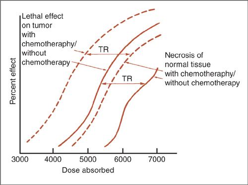
FIGURE 12.1.   Theoretic curves for tumor control and complications as a function of radiation dose both with and without chemotherapy. TR, therapeutic range, or the difference between tumor control and complication frequency.

Source: Reprinted from Perez CA, Thomas PRM. Radiation therapy: basic concepts and clinical implications. In: Sutow WW, Fernbach DJ, Vietti TJ, eds. Clinical Pediatric Oncology. 3rd ed. St. Louis: Mosby; 1984:167, with permission from Elsevier.

When it comes to actually treating patients, physicians do not actively engage in the above mental exercise. However, the basic concepts of the log kill model are reflected in the administered treatments. Consider, for example, curative therapy for cervical cancer. Radiation oncologists begin treatment planning by first identifying the targets GTV (gross target volume) and CTV (clinical target volume) (Fig. 12.2). The CTV is any region that has a high likelihood of harboring malignancy, but otherwise appears normal. For cervical cancer, this could be normal-sized pelvic and possibly paraaortic lymph nodes or an area of positive margin. The CTV typically requires a lower dose of radiation for control, ranging from 45 to 54 Gy. The GTV is defined as any disease that is identified either radiographically or by physical exam, and requires a higher dose of radiation, such as 80 to 90 Gy, in cervical cancer patients. Attaining these doses of radiation while respecting normal tissue tolerance is not feasible with external beam radiation therapy alone and brachytherapy is required. If a patient undergoes a hysterectomy where bulk tumor is removed, then there is not a GTV and brachytherapy is often not needed. So, while the cell kill model is of little practical importance, it is used nonquantitatively for almost every patient receiving radiation treatments.

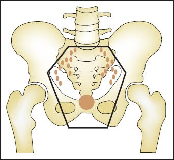
FIGURE 12.2.   Target definition in radiation treatment planning for cervical cancer. The solid circle represents the gross target volume (GTV), which is the cervical primary defined both clinically and radiographically. The clinical target volume (CTV) is the pelvic lymph nodes, which have a high probability of at least microscopic involvement. The planning target volume (PTV) is shown as the outer solid line and represents the margin added to the CTV to account for organ motion and daily setup error.

Cell Survival Curves

The log cell kill model describes cell kill in very simplistic terms such that a given radiation dose will kill a certain percentage of cells and that a tumor receiving a fractionated course of radiation gets progressively smaller with time. This approach looks at behavior in a population of cells, which is practical, but gains very little insight into events at the molecular level. The reason is that measuring the diameter of the tumor is not a very accurate way of estimating cell kill. Additionally, tumor cells may have undergone clonogenic cell death, wherein they are still present but unable to reproduce. Therefore, one does not necessarily have to kill all cancer cells in order to achieve cure if the remaining ones are unable to reproduce.

In order to understand events at the molecular level, one needs to accurately measure cell kill. The technique used most commonly first involves creating a suspension containing the target population of cells at a known concentration (Fig. 12.3). An aliquot with a known number of cells is plated on agarose growth media and allowed to incubate. As one would expect, not all the cells successfully form a colony, and so plating efficiency must be calculated by dividing the number of formed colonies by the starting number of cells. The experiment is repeated, but after plating and before incubation, the petri dish is irradiated. The number of colonies formed is divided by the starting number of cells, which is then divided by plating efficiency to yield the ratio of surviving cells. This experiment is repeated over a range of doses of radiation and under various conditions to yield a cell survival curve. The first feature to notice about a cell survival curve is that it uses a logarithmic scale on the y-axis such that as survival approaches 0, the curve goes to negative infinity. The benefit of plotting the data on a logarithmic scale is that, visually speaking, we are able to interpret whether the events driving cell kill are simple or complex. Consider the analogy of a completely different process, such as the decay of a pure radioisotope over time. Plotting this on a linear scale over time would yield an exponential curve, which is difficult to interpret. However, plotting this on a logarithmic scale would yield a perfect straight line, indicating that a single isotope is involved. Consider a slightly more complex situation where the decay is represented by 2 radioactive isotopes with similar half-lives. Plotting this on a linear scale would also reveal an exponential curve, which is unrevealing by inspection. However, creating a plot on a logarithmic scale would yield 2 lines superimposed on one another, clearly indicating that 2 radioisotopes are involved.

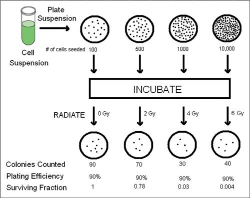
FIGURE 12.3.   Cell culture technique used to generate a cell survival curve. A cell suspension is used to plate Petri dishes with a known number of cells, which are subsequently irradiated. Viable cells will form colonies after incubation. The number of viable cells divided by the plating efficiency is used to calculate the surviving fraction. The experiment is repeated over a wide range of doses to produce the cell survival curve.

Two theoretical experimental cell survival curves are shown in Figure 12.4 under LDR (low-dose-rate) and HDR (high-dose-rate) radiation conditions. The curve for LDR is best fit by a straight line, while the HDR curve is shown to have 2 components, an earlier linear component mirroring the LDR curve followed by a quadratic component. At higher doses of radiation, the HDR curve always has a higher proportion of cell kill than the LDR curve for any given dose.

The rate at which radiation is delivered causes dramatic differences in the shape of the cell survival curve. This is best described by considering the linear-quadratic model with DNA as the lethal target. The evidence for DNA as one of the targets for radiation is substantial: (a) incorporation of radioactive tritium into DNA causes cell death at greater rates than cytoplasmic tritium (2); (b) halogenated pyrimidines, when present in DNA, increase the cell’s inherent radiosensitivity in an amount proportionate to the degree of incorporation; (c) a correlation between radiation, DNA double-stranded break repair, and clonogenic survival has also been observed; (d) the concentration of DNA in the nucleus correlates positively with radiosensitivity (3); (e) microirradiation techniques have shown the nucleus to be the most radiosensitive organelle (4).

In most instances, radiation must cause DNA damage that results in a net loss of genetic material, thereby causing a lethal outcome. Radiation exerts most of its deleterious effects by causing breaks in the DNA backbone. Figure 12.5 shows possible outcomes of photon interaction with the DNA backbone. Because DNA is composed of a double helix with multiple local base pairs acting cooperatively, a single-strand nick is thought to be inconsequential and is repaired by the cellular machinery (Fig. 12.5B). In fact, multiple single-strand nicks can occur, and if they are remote from one another, a normal cell can repair the damage with little chance of a deleterious outcome (Fig. 12.5C). However, 2 opposing single-strand breaks locally disrupt cooperativity, and a double-stranded break (DSB) develops.

FIGURE 12.4.   Cell killing by radiation is largely due to aberrations caused by breaks in 2 chromosomes. The dose-response curve for high-dose-rate irradiation is linear-quadratic: the 2 breaks may be caused by the same electron (dominant at low doses) or by 2 different electrons (dominant at higher doses). For low-dose-rate irradiation, where radiation is delivered over a protracted period, the principal mechanism of cell killing is by the single electron. Consequently, the LDR survival curve is an extension of the low-dose region of the HDR survival curve.

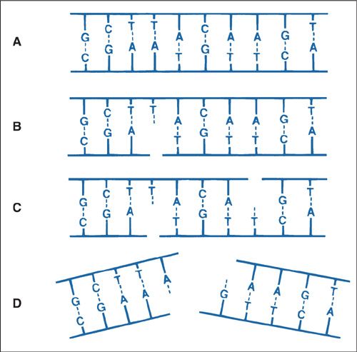
FIGURE 12.5.   Diagrams of single- and double-strand DNA breaks caused by radiation. A: Two-dimensional representation of the normal DNA double helix. The base pairs carrying the genetic code are complementary (i.e., adenine pairs with thymine, guanine pairs with cytosine). B: A break in one strand is of little significance because it is readily repaired, using the opposite strand as a template. C: Breaks in both strands, if well separated, are repaired as independent breaks. D: If breaks occur in both strands and are directly opposite or separated by only a few base pairs, this may lead to a double-strand break, where the chromatin snaps into 2 pieces.

Source: Courtesy of Dr. John Ward. From Hall EJ. Radiobiology for the Radiologist. 4th ed. Philadelphia, PA: JB Lippincott Co.; 1994, with permission.

Once a DSB develops, the cell attempts repair by rejoining the cut ends, as shown in Figure 12.6. There are 2 possible outcomes with repair of the DSBs: the lethal outcomes are shown at the top of Figure 12.6, wherein the chromosomes rearrange such that a portion lacks a centromere, an acentric fragment. When the cell undergoes mitosis, these acentric fragments are eventually lost and may be identified in micronuclei, a smaller “subnucleus” found in the cytoplasm in a separate compartment from the chromosomes (5,6,7). The nonlethal outcomes are shown at the bottom of Figure 12.6, where repair results in a reciprocal translocation and preservation of the genetic information. In some instances, the reciprocal translocation results in activation of an oncogene, which may manifest as a malignancy. It is worth noting that a “bystander effect” has been described using microbeam irradiation techniques (8). In this approach, a nanoscale α-particle beam is directed at the nucleus of a single cell. DSBs can be seen to develop in immediately adjacent unirradiated cells. This is just one notable example where classic radiation DNA damage models fail to explain an observation.

With the above information, the differences in the shape of the cell survival curve under HDR verses LDR conditions can be more easily understood. Referring back to Figure 12.4, in the inset is shown the linear-quadratic model depicting 2 DSBs that develop as result of a photon ejecting an electron, which interacts with DNA. Recall from Figure 12.6 that 2 separate chromosomal breaks are necessary for a potentially lethal outcome. Above the quadratic model is the linear model represented as a single ejected electron causing both DSBs and described mathematically by εαD, where ε and α are both constants and D is dose. The important point is that the degree of the linear component of cell kill, also known as α kill, is proportional to D since only one photon/electron is involved. The quadratic model also shows 2 chromosomal breaks. This is caused by 2 separate ejected electrons and is described by εβD², where ε and β are constants and D is dose. Cell kill accounted for by the quadratic model, or β kill, is proportional to D² because 2 photons/electrons are involved. Looking at the HDR curve at low doses of radiation, there is very little β kill; however, at higher doses, the β component increases exponentially because of D². Under LDR conditions, the β component is absent, leaving only α kill. This is best explained by the idea that β kill involves damage to one chromosome and so is more easily repaired provided that the radiation dose rate and rate of DSB formation is not significantly greater than the cell’s repair capacity.

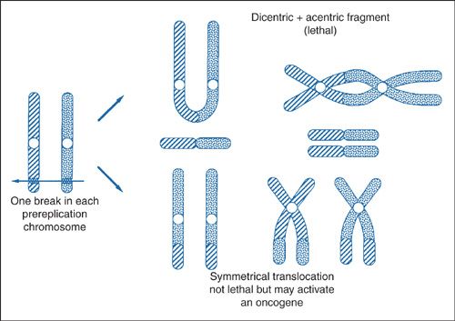
FIGURE 12.6.   Most biologic effects of radiation are due to the incorrect joining of breaks in 2 chromosomes. For example, the 2 broken chromosomes may recombine to form a dicentric (a chromosome with 2 centromeres) and an acentric fragment (a fragment with no centromere). This is a lethal lesion resulting in cell death. Alternatively, the 2 broken chromosomes may exchange broken ends, called symmetrical translocation, which does not lead to death of the cell, but in a few special cases activates an oncogene by moving it from a quiescent to an active site.

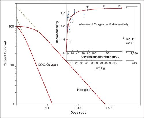
FIGURE 12.7.   Influence of oxygen tension on radiosensitivity. Survival curve for human embryo liver cells in tissue culture irradiated with and without oxygen.

Source: From Johns HE, Cunningham JR. The Physics of Radiology. 3rd ed. Springfield, IL: Charles C Thomas; 1972, with permission.

DNA Damage Repair and the Shape of Cell Survival Curves

The concept that DNA damage repair drives the shapes of cell survival curves is well illustrated by experiments showing the effectiveness of oxygen as a sensitizer. Oxygen is known to chemically modify radiation-induced DNA damage making it irreparable (8). This is known as the oxygen fixation hypothesis. Therefore, under anoxic conditions, DNA damage repair would be expected to increase considerably. Figure 12.7 shows an experiment on cultured human embryo liver cells irradiated under 100% oxygen and nitrogen conditions. Hypoxia causes the cell survival curve to shift to the right and change shape.

Up to this point, the linear-quadratic model has been used to describe cell survival curve experiments. Another way to describe the observations is using the multitarget single hit model, which simply states that multiple targets within a cell must be damaged for a lethal outcome. Therefore, at very low doses of radiation, there will be nearly 100% survival. The model is described mathematically by Survival = 1– (1 – e^–D/D₀)ⁿ, where D is dose delivered, D₀ is the amount of radiation to achieve approximately 63% cell kill. The parameter n is the extrapolation coefficient or the number of targets in each cell, and is identified by where an imaginary straight line drawn back from the linear portion of the cell survival curve crosses the y-intercept. It is important to note that this model makes no statement about what the targets actually are. Since we already know that the primary target is DNA, which can trigger multiple complicated events such as repair and apoptosis, the multitarget single hit model falls short of perfection. Nevertheless, it is a good model for understanding the general shapes of survival curves. Contrast this model to the single-target single hit model, which states that a cell needs only to sustain a single hit for lethality, and is described mathematically by Survival = e^–D/Do. Therefore, even at very low doses of radiation, there will be cell kill. Note that this model does not have an extrapolation coefficient.

Referring back to Figure 12.7, the cell survival curve under anoxic conditions can be interpreted as having a higher extrapolation coefficient when compared to 100% oxygen. The extrapolation coefficient is shown diagrammatically by following the dotted lines of the survival curves back to the y-intercept. The dotted line crosses the y-intercept at n.

The inset shows a dose–response relationship between oxygen and radiosensitivity. The typical sigmoidal relationship is lost because oxygen is extremely effective at fixing DNA damage even at low pressures. In fact, only approximately 20 mm Hg or 2% to 3% oxygen is required to achieve the maximum oxygen effect. The half-maximum sensitization is typically observed at 3 mm Hg or 0.5% of oxygen.

The linear-quadratic model is stated more explicitly by the following equation:

−ln S = αD + βD²

where S is the surviving fraction and the remaining parameters α, β, and D are the same definitions as above. The formula was used to generate Figure 12.8. The dashed line represents the α component and is generated by extrapolating the initial slope of the curve to higher doses of radiation. The point at which the α and β kill are equal is shown, and the dose at which this occurs is called the α/β ratio. It is worth noting that the α/β ratio is a bit of a misnomer, as ratios typically are unitless values. However, α/β has the units of Gy²¹. The α/β ratio for early side effects is thought to be higher, around 10 Gy^–1, than for tumor control and late side effects, which is around 3 Gy^–1.

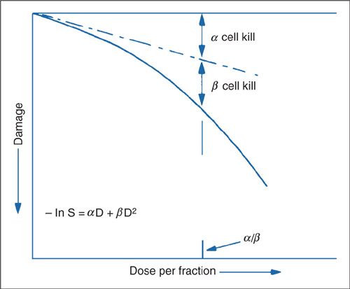
FIGURE 12.8.   At a dose equal to the α/β ratio, the log cell kill due to the α process (nonreparable) is equal to that due to the β process (reparable injury): α/β is thus a measure of how soon the survival curve begins to bend over significantly.

Source: Reprinted from Fowler JR. Fractionation and therapeutic gain. In: Steel GG, Adams GE, Peckham MJ, eds. Biologic Basis of Radiotherapy. Amsterdam: Elsevier Science; 1983:181–194, with permission from Elsevier.

Biologically Equivalent Dose

It is clear from Figure 12.4 that both the total dose of radiation and how fast it is delivered can produce very different outcomes. The same holds true for fractionated courses of radiation. For example, 16 Gy delivered in a single treatment, as is the case for radiosurgery, can sterilize a small tumor of cancer cells. However, the same treatment delivered over 8 days would be clinically insignificant. Figure 12.9 shows theoretical cell survival curves for early and late reactions under two separate experimental conditions, single fraction and multifraction regimens. Note that by breaking up the radiotherapy in fractions, the shoulder of the cell survival curve is repeated. A formula that would normalize a biologic endpoint under various dose fractionation schemes is necessary. The linear-quadratic equation can be used to derive an equation to be used as a guide to predict various biologic endpoints and is given by the following equation:

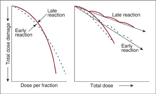
FIGURE 12.9.   Difference in cell survival curves for acute and late radiation effects with single or multifractionated doses of irradiation.

Source: Reprinted from Fowler JF. Fractionation and therapeutic gain. In: Steel GG, Adams GE, Peckham MT, eds. Biologic Basis of Radiotherapy. Amsterdam: Elsevier Science; 1983:181, with permission from Elsevier.

BED = D[1 + d/(α/β)]

A good example where the formula aided the design of a randomized trial, RTOG 8305, is shown below (9). This trial investigated two different fractionation schemes in the treatment of metastatic melanoma.

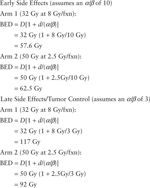
In this instance, the BED calculations predict that arm 1 will have slightly more early and late side effects but better tumor control. BED calculations are used as a guide for determining doses. Oftentimes the calculations do not translate directly into the clinical setting outcomes. For example, RTOG 8305 was not able to detect a difference between the two dose fractionation schemes.

The Cell Cycle

The cell cycle is an ordered set of events, resulting in cell growth and division into two daughter cells. The steps pictured in the middle of Figure 12.10 are G₁-S-G₂-M. The G₁ stands for “gap 1,” and S phase stands for “synthesis” and is the point at which DNA replication occurs. Late S phase is the most radioresistant phase of the cell cycle since the DNA repair machinery for replication can also repair radiation damage. The G₂ stage stands for “gap 2,” and M phase stands for “mitosis” and is when nuclear division occurs. M phase is also the most radiosensitive phase of the cell cycle since this is an all or nothing event. In other words, once the cell enters into M phase, it will attempt to complete this phase of the cycle without arresting. Therefore, any DNA damage caused generally will be passed along to the daughter cells and may be fatal. This is one important reason why rapidly dividing cells such as cancers are radiosensitive. Not shown in Figure 12.10 is G₀, which is a stable state of the cell and is typically observed with well-differentiated cells that have reached end stage of development and are no longer dividing (i.e., neuron).

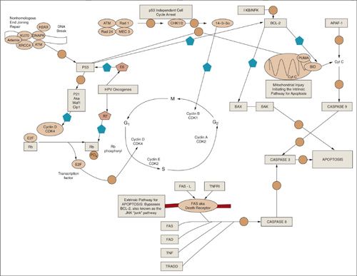
FIGURE 12.10.   The cell cycle and important molecular biologic pathways driving cell cycle arrest, aptoptosis, and survival are shown. The solid pentagon denotes a net inhibitor step and the open circle indicates a downstream step.

There are three major classes of proteins that orchestrate the cell cycle in mammalian cells: (a) cyclins, (b) cyclin-dependent kinases (cdk in mammals, cdc in yeast), (c) proteins that regulate (a) and (b). Cyclins are generally synthesized and degraded for each phase of the cell cycle. Alone they have no intrinsic enzymatic activity; rather, they bind to and activate cdks. Monomeric cdks are protein kinases that are inactive and require association with a specific cyclin and phosphorylation of a series of conserved threonine residues to become active. Cyclin D/cdk4 is involved with G₁ phase of the cell cycle, cyclin E/cdk2 with G₁ to S phase, cyclin A/cdk2 with S to G₂, and cyclin B/cdk1 with M.

Cellular Response to Radiation

When a cell is irradiated, there are, in general, four possible outcomes. The cell can survive, undergo apoptosis, undergo a mitotic death, or senesce. Survival requires cell cycle arrest and repair of damaged DNA. Apoptosis requires intact molecular biologic pathways that favor an ordered process of programmed cell death within hours of exposure to radiation. Unfortunately, most tumors have mutations in these pathways, but in malignancies such as lymphoma where these pathways are intact, the tumors can respond after only a couple of radiation treatments. Cells that die a mitotic death undergo a catastrophic event when trying to replicate and so responses may take days. Tumors that die via this mechanism are more radioresistant and result in necrotic masses on imaging after completing a course of radiation. Senescence is a state in which proliferation is irreversibly arrested and the cell may eventually die. Note that senescence is a metabolically active state, which is different from G₀, which is typically metabolically inactive.

Inherent to the cell is a type of thermostat, which influences the radiation responses to favor any of the above processes. Protooncogenes are regulator proteins that, due to either overexpression or mutation, have a higher activity level, thereby promoting unregulated division. Because this mechanism is a net gain of function, only one allele needs to be affected in order to see phenotypic expression. Tumor suppressor genes keep the cell cycle in check, and so loss of function of both alleles is typically required for dysregulation to be observed.

Cell Cycle Arrest

As previously mentioned, when a cell is irradiated, repair of the DNA backbone is attempted, and in order for this process to occur the cell cycle must typically arrest. There are two prototypical points in the cell cycle during which arrest occurs: G₁ and G₂ (10,11). A major regulator of the cell cycle is the transcription factor p53, which is a tumor-suppressor gene that has many pathways both upstream and downstream and is important for G₁ arrest (Fig. 12.10) (12). For example, breaks in the DNA backbone are rejoined via the nonhomologous end-joining (NHEJ) repair mechanisms (top left of Fig. 12.10) (13). One critical gene, the ataxia telangiectasia gene (ATM) has a net positive regulatory effect on p53, which, via p21 (CCDKN1A), has a net inhibitory effect on cyclin D/cdk4, thereby favoring arrest. This is the p53-dependent pathway of cell-cycle arrest. An alternative pathway, independent of p53, operates via chk1/2 and 14-3-3α gene products and has a net inhibitory effect on cyclin B/cdk1, which promotes arrest during G₂ (14).

Retinoblastoma Gene, E2F, and Human Papillomavirus

Retinoblastoma protein (Rb) is another critical regulator of the G₁ phase of the cell cycle (15). This gene is located on chromosome 13 and mutations can cause a number of tumors, the earliest of which to manifest is retinoblastoma. Knudson et al. developed the two-hit hypothesis for the inheritance pattern of this disease (16). He recognized that there were 2 forms: (a) sporadic, which comprises 60% of the cases of retinoblastoma, whereby mutations occur as random events in both alleles. Patients typically have unilateral disease and a marginal risk for developing second malignancies in response to radiation; and (b) Inherited, where a germ-line mutation results when an abnormal allele is inherited from a parent. Patients with this form of retinoblastoma are more likely to develop bilateral disease and have a profound sensitivity toward developing radiation-induced second malignancies. Rb acts by binding and inhibiting E2F, a transcription factor essential for G₁. Phosphorylation of Rb results in release of inhibition of E2F and subsequent cell cycle progression. Human papillomavirus gene product produces an oncogene, E7, which binds to Rb and releases inhibition of E2F, thereby promoting cell division (17).

Apoptosis

Apoptosis can begin in 2 distinct manners: (a) extrinsic pathway, where the apoptotic stimulus occurs extracellularly, or (b) intrinsic pathway, where the cascade of events is contained intracellularly. Figure 12.10 shows both pathways converging on caspase 8 (cysteine aspartic acid-specific proteases). Caspases are expressed as inactive precursors (procaspases), which are proteolytically cleaved to an active state following an apoptotic stimulus. Upstream from caspase 8, the pathways diverge. The extrinsic pathway begins by binding of a specific ligand such as Fas-L or tumor necrosis factor (TNF) to a membrane-bound death receptor. The intrinsic pathway, on the other hand, requires disruption of the mitochondrial membrane and release of mitochondrial cytochrome to the cytoplasm. Cyt c then combines with 2 other cytosolic protein factors, Apaf-1 (apoptotic protease activating factor-1) and procaspase-9, to promote the assembly of a caspase-activating complex termed the apoptosome, thereby promoting the apoptotic caspase cascade. Bcl-2 and its family member proteins are important regulators of apoptosis. Bcl-2 is antiapoptotic by inhibiting proapoptotic factor bax and inhibiting the release of cyt c into the cytoplasm. p53 is an important inhibitor of bcl-2. All of these pathways interact to determine whether a cell will survive or apoptose in response to an insulting stimulus such as radiation.

Radiation Effects on Embryo and Fetus

In Utero Exposure to Ionizing Radiation

There are 2 models that describe the negative clinical sequelae of exposure to radiation to a developing fetus or embryo. (a) Deterministic effects describe how radiation affects a large population of cells resulting in end organ damage. A large number of cells must die in order to induce organ failure. As such, deterministic effects tend to have a sigmoidal dose–response relationship with a threshold dose. As long as the threshold dose is respected, there is very little chance of a given toxicity. (b) Stochastic effects describe events at the cellular level and how radiation induces malignancies. Stochastic effects have more of a constant, steep dose-response relationship. As such, there is no threshold dose; that is, exposure to even miniscule amounts of additional radiation theoretically increases the chance of inducing a malignancy.

Deterministic Effects—End Organ Damage and Failure

The most sensitive phase of the cell cycle to ionizing radiation is M phase because little repair to the DNA backbone occurs during this period. Most of the cell molecular machinery is geared toward completing mitosis and any DNA double-stranded breaks are passed along to the daughter cells and are typically fatal. Since embryos and fetuses are composed of rapidly dividing cells, they are exquisitely sensitive to radiation and exhibit an extremely low threshold dose. Gestational age is also a key determinant when predicting outcomes of radiation exposure. As Figure 12.11 shows, exposure of several gray during the first 1 to 2 weeks of gestation (peri-implantation stage) results in loss of the embryo. However, if the embryo survives the insult, it will go on to develop without obvious abnormalities. This phenomenon is termed the “all or nothing effect.” During weeks 2 to 6, the period of organogenesis is occurring and exposure at this point results in congenital anomalies, neonatal death, and temporary growth retardation. Doses as low as 2 Gy have a 70% mortality. The fetal period occurs beyond 6 weeks and exposure results in permanent growth retardation. Irradiation during weeks 4 through 16 may produce severe eye, skeletal, and genital organ abnormalities as well as microcephaly and mental retardation. According to the Japanese survival data, the risk is approximately 40% per gray. Exposure during weeks 16 through 20 may cause a less severe form of stunting of growth, microcephaly, and mental retardation. After 30 weeks, low doses of radiation do not typically result in gross abnormalities.

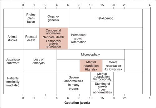
FIGURE 12.11.   Summary of the effects of radiation on the developing embryo and fetus from 3 principal sources: medical radiation, laboratory animal studies, and survivors of the atomic bomb attacks on Nagasaki and Hiroshima. The animal studies indicate a wide range of structural abnormalities during organogenesis, whereas the principal effect observed in humans is reduced head diameter with or without severe mental retardation.

Source: Modified from Hall EJ. Radiobiology for the Radiologist. 4th ed. Philadelphia: JB Lippincott Co.; 1994, with permission.

Stochastic Effects—Cancer Induction

The Oxford Survey by Kneale and Stewart suggested that there was an association between leukemia risk and in utero exposure to diagnostic X-rays (18). Doll and Wakeford summarized the data with the following general conclusions: Low-dose irradiation increases the risk of childhood malignancies, particularly in the third trimester (19). An X-ray exam increases the risk by approximately 40% above the spontaneous rate. Doses as low as approximately 10 mGy increase the risk, and the excess absolute risk is around 6% per gray. Solid tumors have a longer latency period of approximately 20 to 40 years, whereas leukemias have an average latency of around 7 years. When counseling the pregnant patient or worker, it is important to let them know the magnitude of and potential for side effects. According to the International Council of Radiation Protection (ICRP) Publication 84, doses less than 1 mGy may be considered negligible, which is the approximate dose of normal background radiation (20). Exposures above 1 mGy require a more in-depth discussion with the patient. ICRP Publication 84 provides detailed risk assessments and counseling guidelines for in utero exposure.

Occupational Exposure

Once pregnancy has been declared, the employee is encouraged to formally inform her employer. Further, the radiation safety officer should interview her, her employment should be evaluated for exposure history, and steps should be taken to minimize exposure. The National Council on Radiological Protection recommends that the embryo/fetus have limited exposure to less than 0.5 Sv/month (21).

INTRODUCTION TO RADIATION PHYSICS

Radiation physics is the study of the interaction of radiation with matter. In the treatment of patients with radiation, this matter is either tumor tissue or normal tissues such as the skin, the internal organs, or the supporting tissues and structures.

Units Used in Radiation and Radiation Therapy

Radiation is an abbreviation for electromagnetic radiation. It can occur in numerous forms. The most common forms used in radiation therapy are X-rays, γ-rays, and electrons. X-rays and γ-rays are also known as photons or packets of energy and are used to treat most body sites where radiation is deemed efficacious. Other particles or forms of radiation, such as protons, neutrons, and heavier α particles, are less commonly used in radiation therapy except in select clinical situations. Protons, other heavy charged particles, and neutrons have a higher linear energy transfer coefficient when compared to high energy photons and therefore are more efficient at transferring or depositing their energy in tissue. Protons are used increasingly in the treatment of prostate cancers, choroidal melanomas, skull base and paraspinal tumors, and pediatric tumors. Neutrons have been used for salivary gland tumors, sarcomas, and prostate cancers. Protons are positively charged particles that can be accelerated in an electric field to high energies. The primary characteristic of a proton beam is its Bragg peak. The Bragg peak describes at what depth the majority of a proton’s energy is deposited. Prior to the depth of the Bragg peak, only a very small amount of the proton energy is deposited. The Bragg peak depth is determined by the energy of the incident protons and covers only very small width of tissue at that depth. In order to cover more tissue, the energy of the incoming proton beam is varied. The net dose deposition results in a low entrance dose and a finely controlled width of treatment dose at depth. This makes proton treatments an excellent choice for the treatment of tumors adjacent to critical structures. Neutrons are relatively massive uncharged particles that can be generated by cyclotrons. Poor treatment geometry and dose distributions have limited the enthusiasm for neutron beam therapy (22).

Stay updated, free articles. Join our Telegram channel

Join