Fig. 4.1
Growth of long bones. Schematic diagram illustrating the growth of long bones: (a) Longitudinal growth occurs due to hypertrophic differentiation of growth plate chondrocyte. (b) Bone morphology is maintained by osteoclast-directed metaphyseal in-waisting. (c) Bone remodelling removes the mineralised cartilage scaffold and deposits new trabecular bone. (d) Diaphyseal bone diameter is increased by osteoblast-mediated periosteal apposition
Long bones develop through a process of endochondral ossification [14]. Linear growth occurs at the epiphyseal growth plates that lie between the epiphyses and metaphyses at either end of long bones. The growth plate chondrocytes form highly organised columns divided into three distinct zones; the reserve zone nearest the epiphysis, the proliferative zone and the hypertrophic zone nearest the metaphysis. Reserve zone chondrocytes begin to proliferate in discrete columns extending the growth plate. Following a period of proliferation chondrocytes then undergo hypertrophic differentiation, expanding to ten times their previous volume and producing angiogenic factors. These factors lead to vascular invasion and apoptosis of the hypertrophic chondrocytes. The invading blood vessels also bring osteoclast and osteoblast precursors which convert the mineralised cartilage scaffold into new bone through remodelling [15]. At cessation of growth, chondrocyte proliferation progressively slows ultimately leading to the fusion of the metaphysis and epiphysis.
During longitudinal growth the processes of bone modelling optimise the shape of skeletal elements to their required function. In bone modelling osteoclastic bone resorption and osteoblastic bone formation are not coupled but rather actively coordinated to dynamically reshape the bone. In long bones the growth plate has the widest cross section and the diaphysis the narrowest, with the intervening tapered region termed the metaphysis. As linear growth occurs osteoclasts resorb the periosteal surface of the metaphysis (metaphyseal in-waisting) and osteoblasts lay down new bone on its endosteal surface, thus reshaping the metaphysis into the diaphysis. Importantly, anti-resorptive agents can interfere with this process, leading to club-shaped metaphysis and bone deformities known as undertubulation [16]. During growth, periosteal bone formation (periosteal apposition) also increases the diaphyseal diameter and cortical thickness is determined by the net balance of this periosteal apposition and concurrent endosteal resorption [17].
What Are the Aims of Drug Therapy?
The aim of drug therapy for osteoporosis is covered in detail in other chapters in this book, but in essence it is to enable the skeleton to achieve maximal functional capacity. Overall the intention then is to reduce the frequency of fractures, control pain and improve linear growth.
Prior to 1998 pharmacological treatment for children with fragility fractures was very limited. However, the demonstration that the anti-resorptive bisphosphonates increased BMD and reduced fracture risk in children with osteogenesis imperfecta revolutionised the field [18]. Intravenous bisphosphonates are now considered to be the mainstay of treatment for children with osteoporosis (see Chap. 5). More recently, the alternative anti-resorptive therapies have been developed and now RANKL antibody (denosumab) and cathepsin K inhibitors are also beginning to be used in children [19].
Benefits of Anti-resorptives
Anti-resorptive therapies act by impeding osteoclastic removal of bone while still allowing osteoblastic bone formation to continue. In the growing skeleton, the effect of anti-resorptive therapy on increasing bone mass is amplified and related to the rate of growth, modelling and remodelling. This leads to increased trabecular bone and cortical thickness [20]. Osteoclasts have a major role in modelling trabecular bone adjacent to the growth plate. Anti-resorptives interfere with this process and result in the retention of trabecular bone and mineralised cartilage. This increases bone mineral content (BMC) and improves mechanical strength to this region of the bone. This increase in trabecular bone is particularly beneficial in the vertebral bodies and children treated with bisphosphonates show reduced vertebral compression fracture and improved healing. The effects of anti-resorptives on growth remain uncertain. However, improvements in height Z-scores in some studies suggest that treatment may also improve growth [18]. By contrast, the reduction in long bone fracture risk following anti-resorptive treatment is thought to be due to reduced endosteal resorption and thus an increased diaphyseal cortical thickness. Bisphosphonates have been used to reduce pain in fibrous dysplasia [21] and several uncontrolled trials have reported bisphosphonate-related pain relief; however, this has not yet been confirmed by randomised controlled trials.
Long-Term Adverse Effects of Anti-resorptives
During growth, treatment with anti-resorptive medication impairs bone modelling and so inhibits the normal metaphyseal periosteal resorption. This results in reduced metaphyseal in-wasting and club-shaped long bones. Anti-resorptive treatment also impairs bone remodelling resulting in altered bone structure and quality. Impaired trabecular remodelling below the growth plate results in retention of calcified cartilage [20]. Although adverse effects from retained calcified cartilage have not been directly demonstrated, it is thought to increase the brittleness and reduce the toughness of trabecular bone. Anti-resorptive treatment results in thicker and mechanically stronger cortical bone but the concomitant reduction in microdamage repair is likely to result in bone of inferior quality.
In addition to the adverse structural consequences of anti-resorptives, concerns remain regarding the retention of bisphosphonates within the skeleton after cessation of treatment. This may be clinically important as the bisphosphonate can be re-released during periods of high bone turnover such as pregnancy and lactation. This consideration however remains only a theoretical risk as no adverse events have been reported. Nevertheless, it may be prudent to use the lowest dose of bisphosphonate to achieve the desired clinical outcome. As for any therapeutic intervention, the acute and long-term benefits and risks need to be carefully considered, and continued monitoring of treatment is essential for the optimisation of therapy and safeguarding against potential adverse effects.
How Do We Monitor the Effects of Drugs on Bone Physiology?
When monitoring bone health, a number of different properties of bone and bone metabolism can be measured that reflect the state of the skeleton as a whole, or that of individual bones or bone types. There are various different techniques that can be used for this evaluation, each with benefits and limitations that must be taken into account when using them in children with bone disease. The most common techniques for monitoring bone health are discussed below.
X-Ray Analysis
The oldest and simplest way of monitoring the skeleton in children and adolescents is to use plane X-ray. While this does not yield information regarding material properties or micro-geometry, much information can still be gained. The gross morphology, size and bone age can easily be determined and fractures and deformities readily identified. Moreover, annual X-ray of the lateral spine can be particularly helpful in monitoring vertebral compression fractures (see Fig. 4.2) since vertebral morphometry can be used to quantify the degree of compression and healing [22]. A major drawback to the use of X-ray is the relatively high radiation doses involved. These can be as high as 0.7 mSv for lumbar spine X-rays, significantly higher than other modalities [23].
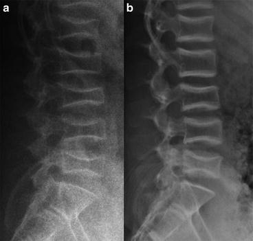
Fig. 4.2
Monitoring vertebral fracture healing during treatment using X-rays. Lateral X-rays of lumbar vertebral compression fractures in a 13-year-old boy with osteoporosis. (a) Prior to treatment with pamidronate. (b) After 2 years of treatment. Note how the shapes of the vertebrae have remodelled and healed. (Courtesy of Dr. J. Allgrove, Royal London Hospital, UK)
Abnormal vertebral geometry is quantitated by identifying the four corners of each vertebral body and the mid-points of the end plates and then determining the distances between these six points. The anterior, posterior and mid-point heights, the lower vertebral length and the vertebral height ratios are calculated. The concavity index is determined by calculating the average ratio between the mid-point height and the posterior height for each of the first four lumbar vertebrae (L1–L4). In general, the less tall and the more concave the vertebrae the worse its vertebral shape. The monitoring of paediatric compression fractures by this method is well established and it commonly forms part of annual screening protocols [24].
Dual-Energy X-Ray Absorptiometry
Dual-energy X-ray absorptiometry (DXA) is the most widely used method for assessing bone health in children due to its availability, speed, low cost, non-invasive nature and low radiation dose, and is currently considered to be the “gold standard” for bone densitometry. Nevertheless, to prevent incorrect interpretation there are a number of important issues that must be considered when DXA is used for diagnostic or monitoring purposes. These are discussed in detail below.
A DXA system consists of a scanning X-ray source, an X-ray detector that records absorption at both high and low energy X-rays and a computer system to analyse this data. DXA analysis makes the assumption that the body is divided into two tissue compartments; bone and non-bone. The high and low energy X-rays are differentially absorbed by these two compartments allowing the conversion of the absorption data into mass values for bone and non-bone. This can be done for the whole body or for selected regions such as the lumbar spine, proximal femur or distal radius. DXA can also be utilised for the assessment of other tissues of differing densities, such as lean body mass and fat mass, thus providing important information about body composition.
DXA results are expressed in terms of either BMC or BMD. These parameters are calculated for a selected region of interest (ROI) that consists of bone tissue with the two-dimensional bone area (BA) measured in cm2. The X-ray attenuation within this ROI is then compared to a reference standard of known mineral density, thus allowing the BMC in grams to be calculated for each pixel. The total BMC for the ROI is then calculated by summing all these pixel values. The BMD of the ROI in g/cm2 is calculated by dividing the BMC by the bone area (BMD = BMC/BA). Importantly, DXA does not measure the true bone BMD as it is a linear absorption method and so can only provide a two-dimensional analysis of a three-dimensional structure. This means DXA quantifies the “areal” BMD or aBMD rather than the volumetric BMD or vBMD. Thus, in large bone aBMD will overestimate vBMD, while in a small bone it will underestimate it (see Fig. 4.3). In adults, bone size is constant and therefore this does not represent a major problem. However, the rapid increase in bone size in childhood means that the aBMD estimation of vBMD will progressively increase with age and this must be taken into account. Thus, DXA parameters should always be compared to normative range values for the appropriate age, rather than making direct comparisons with previous values. Since bones grow at different rates, comparisons between different ROIs are also inherently more difficult. To ensure accuracy and reproducibility of DXA measurement it is important that the position of the child and the selection of the ROI are standardised. The most commonly used ROIs include (1) total skeleton minus head, (2) lumbar spine from L1/L2 to L4 and (3) femoral neck. Total skeleton aBMD is useful for estimating overall bone health while lumbar spine and femoral neck ROIs determine aBMD at the most common fracture sites. Because these DXA parameters are compared to a normative population reference range, poor position or ROI selection can invalidate the findings (see Fig. 4.4). DXA analysis software uses algorithms to distinguish between bone and non-bone compartments when selecting the ROI. As children have a lower BMD than adults the use of an adult algorithm will result in an inaccurate ROI with the exclusion of bone with lowest density and thus an overestimation of BMD [25]. It is, therefore, important to use a modified child-specific algorithm for DXA analysis.
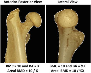
Fig. 4.3
The effect of bone size on areal BMD. A small and a large bone are schematically represented by the small and large cubes. Although both bones have identical volumetric BMD, the larger bone will have a higher areal BMD as measured by DXA
Fig. 4.4
Consistent positioning and ROI selection are required when comparing DXA scan results. The same femoral head is shown in both the lateral and AP orientations. While the volumetric BMD clearly remains the same, the change in position has altered the bone area, thus changing the areal BMD as measured by DXA
DXA data must be compared to a normative reference range for age before they can be interpreted. In adults the results are normally reported as a T-score, defined as the number of standard deviations from the population peak adult BMD. The World Health Organisation uses this T-score to define osteoporosis and osteopenia (T < −2.5 and T < −1, respectively) [26] but clearly such a definition is not useful in children, as they have not yet reached peak bone mass. Instead the Z-score can be used, defined as the number of standard deviations from the average population BMD at the patient’s age. To accurately determine the Z-score an appropriate reference range is therefore required. It is important to select the correct reference database and not simply to use reference data provided by the manufacturer. Previously, obtaining appropriate paediatric reference ranges was a major problem, but there is now an increasing number of databases available (Table 4.1). However, there are also many demographic factors that must be considered when selecting appropriate DXA reference data including gender, ethnicity, age, height, weight and Tanner stage. When selecting a reference range it is important to also consider the ROIs studied, ROI selection algorithms, scanner brand, scanner model and software version.
Table 4.1
Available reference data for the analysis of paediatric bone
Year | Population (M/F) | Age range | Ethnicity | Location | Machine | Input | Output | References |
|---|---|---|---|---|---|---|---|---|
DXA | ||||||||
1990 | 70/65 | 1–15 years | White | France | QDR-1000 | Gender, age, Ht, Wt, Tanner | LSBMD | [44] |
1991 | 109/98 | 9–21 years | White | Switzerland | QDR-1000 | Gender, age, Tanner | LSBMD, LSBMC, FNBMD, FNBMC | [45] |
1991 | 84/134 | 1–19 years | Mixed | USA | QDR-1000 | Gender, age, Tanner, Wt | LSBMD | [46] |
1992 | 28/29 | Newborn | White | France | – | GA, Ht, Wt, SA | LSBMD, LSBMC | [47] |
1992 | 22 | 1–24 months | White | France | – | GA, Ht, Wt, SA | LSBMD, LSBMC | [47] |
1993 | 86/68 | 5–18 years | White | Spain | – | Gender, Tanner | TBBMC | [48] |
1995 | 137/128 | 4–26 years | White | Australia | Lunar DPX | Gender, age | TBBMC | [49] |
1996 | 110/124 | 8–17 years | White | Canada | QDR-2000 | Gender, age | LSBMC, LSBMD, FNBMC, FNBMD, TBBMD, TBBMC | [50] |
1996 | 82/68 | GA 27–42 | White, Black | USA | QDR-1000 | Wt | TBBMC, TBBMD, TBBA | [51] |
1997 | 169/234 | 4–20 years | White | Netherlands | Lunar DPXL/PED | Gender, age, Tanner | TBBMC | [52] |
1997 | 297/0 | 3–18 years | White, Black, Hispanic | USA | QDR-2000 | Age, ethnicity | TBBMC | [53] |
1997 | 0/313 | 3–18 years | White, Black, Hispanic | USA | QDR-2000 | Age, ethnicity | TBBMC | [54] |
1998 | 142/201 | 4–19 years | White | Denmark | QDR-1000 W | Gender, Tanner | TBBMC, TBBMD, TBBA | [55] |
1999 | 193/230 | 9–25 years | White, Asian, Hispanic, Black | USA | QDR-1000 W | Gender, age, ethnicity | LSBMD, LSBMAD, HipBMD, HipBMAD, FNBMD, FNBMAD, TBBMD, BMC/Ht | [56] |
2001 | 0/151 | 9–14 years | White | Netherlands | QDR-2000 | Age, breast stage | LSBMC, LSBMD, FNBMC, FNBMD, FABMC, FABMD | [57] |
2001 | 445/537 | 5–18 years | White, Black, Hispanic | USA | QDR-2000 W | Gender, age, disease status | TBBMC | [58] |
2002 | 188/256 | 4–20 years | White | Netherlands | Lunar DPXL/PED | Gender, age, Tanner | LSBMD, LSBMAD, TBBMC, TBBMD | [59] |
2002 | 117/139 | 3–18 years | White, other | USA | QDR-1000 W/QDR-2000 | Gender, age, Tanner | DFBMD | [60] |
2002 | 107/124 | 5–22 years | White, other | USA | QDR-4500 | Gender, age, Ht, TBBMC | TBBMC, TBBMD, TBBA | [61] |
2003 | 210/249 | 3–30 years | White | Australia | Lunar DPX | Gender, age, Ht | TBBMC/LTM | [62] |
2004 | 0/422 | 12–18 years | Black, non-Black | USA | QDR-4500 W | Age, Wt, ethnicity | LSBMD, LSBMAD, FNBMD, FNBMAD | [63] |
2005 | 284/278 | 5–18 years | White | Poland | Lunar DPXL | Gender, age, Ht | TBBMC, TBBMD, LSBMD, LSBMC, TBBMD/LTM, LSBMD/LTM | [64] |
2007 | 761/793 | 6–16 years | All ethnicities | USA | QDR-4500A, QDR-4500 W, Delphi-A | Gender, age, ethnicity | LSBMD, HipBMD, FNBMD, 1/3RadBMD, TBBMD, TBBMC, LSBMC | [65] |
2007 | 235/200 | 5–18 years | White | UK | QDR Discovery | Gender, age | TBBMAD, LSBMAD, FNBMAD, LSBAforHt, LSBMCforBA, TBBAforHt, TBBMCforBA | [66] |
2009 | 1849/4629 | 7–80 years | Hispanic | Mexico | DXA Lunar DPX NT | Gender, age | TBBMD, LSBMD, FNBMD, HipBMD | [67] |
2009 | 10560/9993 | 8–85 years | White, Black, Hispanic | USA | QDR 4500A | Gender, age, ethnicity, Ht | TBBMC, TBBMD | [68] |
2011 | 992/1022 | 5–23 years | All ethnicities | USA | QDR-4500A, QDR-4500 W, Delphi-A | Gender, age, ethnicity | TBBMD, TBBMC, LSBMD, LSBMC, HipBMD, HipBMC, FNBMC, FNBMD, 1/3RadBMD, 1/3RadBMC | [69] |
2011 | 480/440 | 5–17 years | Indian | India | Lunar DPX Pro | Gender, age, Tanner | TBBMC, TBBMD, TBBA, LSBMD, LSBMAD, FNBMD, FNBMAD | [70] |
2013 | 777/764 | 5–19 years | Chinese | China | Lunar Prodigy DXA | Gender, age | TBBMD, TBBMC, TBBA | [71] |
pQCT | ||||||||
2001 | 185/186 | 6–23 years | White | Germany | XCT 2000 | Gender, age, Tanner | 4%D.Rad—TotBMD, CortBMD, TrabBMD, TotCXSA | [72] |
2001 | 177/185 | 6–23 years | White | Germany | XCT 2000 | Gender, age, Tanner | 65%P.Rad—CortBMC, SSI, strength modulus, polar inertia | [73] |
2001 | 177/186 | 6–23 years | White | Germany | XCT 2000 | Gender, age, Tanner | 65%P.Rad—CortBMD, CortBMC, CortThick, CortA | [72] |
2002 | 107/124 | 5–22 years | USA | XCT 2000 | Gender, age | 20%D.Tib—Periost circ, endost circ, cortBMD | [61] | |
2002 | 177/185 | 6–23 years | White | Germany | XCT 2000 | Gender, age, Tanner | 65%P.Rad—CortBMD, CortThick | [74] |
2005 | 204/274 | 6–40 years | White | Germany | XCT 2000 | Gender, age | 4%D.Rad—TotBMD, TotBMC, TotCXSA, CortThick | [75] |
2008 | 197/219 | 5–18 years | White | USA | – | Age, gender | 4%D.Rad—TotBMD, CortBMD, TrabBMD, TotCXSA | [76] |
2008 | 196/273 | 6–40 years | White | Germany | XCT 2000 | Age, gender | 65%P.Rad—TotBMC, TotBMD, CortBMD, TotCXSA, CortCXSA, SSI | [77] |
2009 | 380/249 | 6–19 years | White | UK | XCT-2000 | Gender, age, Ht | 4%D.Rad—TotBMD, TrabBMD, BA, 50%D.Rad—CortArea, CortThick, CortBMC, BA | [78] |
qUS | ||||||||
1997 | 174/193 | 6–15 years | White | UK | Contact ultrasound bone analyser | Age, gender | Calcaneus—BUA | [79] |
2000 | 287/309 | 6–20 years | White | Netherlands | SoundScan™ Compact | Age, gender, Tanner | Tibia SoS | [80] |
2000 | 262/269 | 6–21 years | White | Netherlands | UBIS 3000 | Age, gender, Tanner | Calcaneus—SoS, BUA (Plus SoS and BUA adjusted for heel width and foot length) | [81] |
2002 | 678/650 | 3–17 years | White | Germany | DBM Sonic 1200 | Age, gender, height, BMI | Finger phalanges—AD-SoS, BTT | [82] |
2003 | 1175/0 | 7–80 years | White
Stay updated, free articles. Join our Telegram channel
Full access? Get Clinical Tree
 Get Clinical Tree app for offline access

| |||||